K-nearest neighbors
Table of Contents
This Nearest-neighbor algorithm defines the neighborhood \(\mathcal(N)\) to contain \(K\) samples from training data.
The algorithm is:
- Find \(K\) samples from training data nearest to \(x_0\) (test predictor).
- Count the occurrence of each class in this neighborhood.
- \(\hat{y}_0\) is given the label with the highest count.
1. Training and testing error rates with \(K\)
The K increases, the training error rate increases. At \(K=1\) the training error rate is the lowest (overfits training data).
But, the testing error decreases with increasing \(K\), reaches a lowest point, and then again shoots up. When \(K=N\), all the test predictions will take the label (majority class in training data).
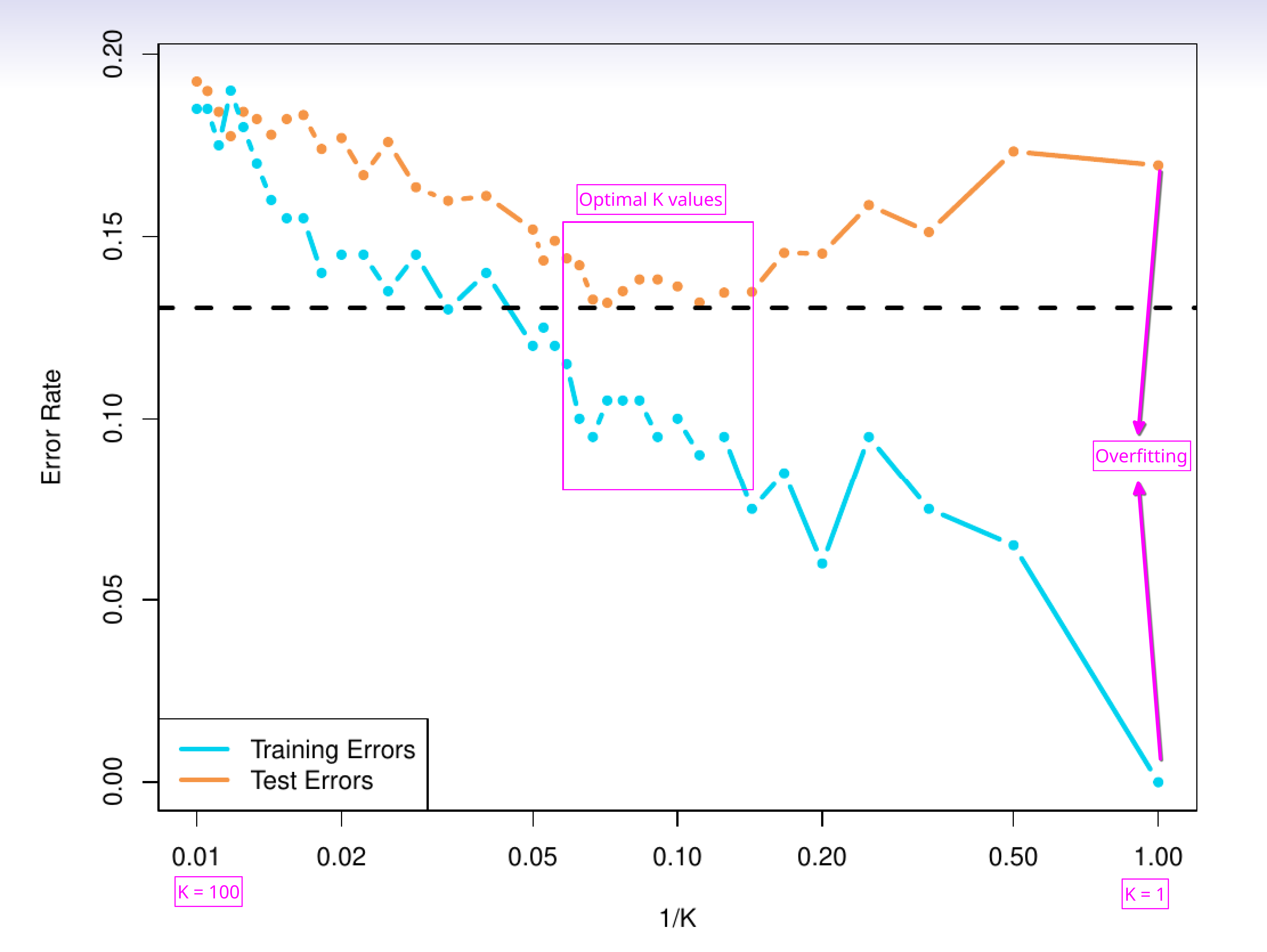
Figure 1: Training and testing error rate trend with \(K\)
2. Decision boundary
The decision boundary is where a classifier decision changes from one class label to another.
In the simulated example demonstrated below, the first image shows Bayes decision boundary. This is available to us only because we know the conditional probability (as the data is simulated). This Bayes decision boundary marks points where the probability of each class is \(0.5\).
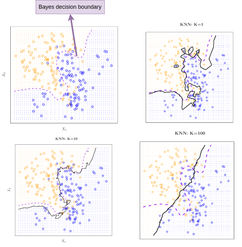
Figure 2: Decision boundary trend with \(K\)